My First Blog Post

Round Robin Scheduling Algorithm

In this blog, we will be learning about the Round Robin scheduling Algorithm.The topics which will be covered are,

• What is Round Robin Scheduling Algorithm?
• Round Robin Scheduling Algorithm
• Code
• Advantages and Disadvantages

What is Round Robin Scheduling?

Round Robin scheduling algorithm is one of the foremost widespread scheduling formula which may really be enforced in most of the operating systems. This is the preventive version of first come first serve scheduling. The Algorithm focuses on Time Sharing. In this formula, each method gets dead in a very cyclic method. A certain time slice is outlined within the system that is termed time quantum. No process will hold the CPU for a long time. The switching is called a context switch. It is probably one of the best scheduling algorithms. The efficiency of this algorithm depends on the quantum value.

Each method present within the prepared queue is allotted the central processing unit for that point quantum, if the execution of the method is completed throughout that point then the method will terminate else the method can return to the prepared queue and waits for consecutive intercommunicate complete the execution.

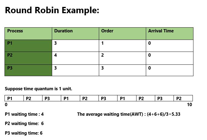
Round Robin Scheduling Algorithm

---

Round Robin could be a central processing unit programming rule wherever every process is appointed a hard and fast slot during a cyclic manner.

• It is easy, simple to implement, and starvation-free as all processes get fair proportion of central processing unit.
• One of the foremost normally used technique in central processing unit programming as a core.
• It is preventive as processes are allotted central processing unit just for a hard and fast slice of your time at the most.
• The disadvantage of it is more overhead of context switching.

Consider the example code

/ C++ program for implementation of RR scheduling 
#include<iostream> 
using namespace std; 
  
// Function to find the waiting time for all 
// processes 
void findWaitingTime(int processes[], int n, 
             int bt[], int wt[], int quantum) 
{ 
    // Make a copy of burst times bt[] to store remaining 
    // burst times. 
    int rem_bt[n]; 
    for (int i = 0 ; i < n ; i++) 
        rem_bt[i] =  bt[i]; 
  
    int t = 0; // Current time 
  
    // Keep traversing processes in round robin manner 
    // until all of them are not done. 
    while (1) 
    { 
        bool done = true; 
  
        // Traverse all processes one by one repeatedly 
        for (int i = 0 ; i < n; i++) 
{ 
            // If burst time of a process is greater than 0 
            // then only need to process further 
            if (rem_bt[i] > 0) 
            { 
                done = false; // There is a pending process 
  
                if (rem_bt[i] > quantum) 
                { 
                    // Increase the value of t i.e. shows 
                    // how much time a process has been processed 
                    t += quantum; 
  
                    // Decrease the burst_time of current process 
                    // by quantum 
                    rem_bt[i] -= quantum; 
                } 
   // If burst time is smaller than or equal to 
                // quantum. Last cycle for this process 
                else
                { 
                    // Increase the value of t i.e. shows 
                    // how much time a process has been processed 
                    t = t + rem_bt[i]; 
  
                    // Waiting time is current time minus time 
                    // used by this process 
                    wt[i] = t - bt[i]; 
  
                    // As the process gets fully executed 
                    // make its remaining burst time = 0 
                    rem_bt[i] = 0; 
                } 
            } 
        } 
  
        // If all processes are done 
        if (done == true) 
          break; 
    } 
} 
  
// Function to calculate turn around time 
void findTurnAroundTime(int processes[], int n, 
                        int bt[], int wt[], int tat[]) 
{ 
    // calculating turnaround time by adding 
    // bt[i] + wt[i] 
    for (int i = 0; i < n ; i++) 
        tat[i] = bt[i] + wt[i]; 
} 
  
// Function to calculate average time 
void findavgTime(int processes[], int n, int bt[], 
                                     int quantum) 
{ 
    int wt[n], tat[n], total_wt = 0, total_tat = 0; 
  
    // Function to find waiting time of all processes 
    findWaitingTime(processes, n, bt, wt, quantum); 
  
    // Function to find turn around time for all processes 
    findTurnAroundTime(processes, n, bt, wt, tat); 
  
    // Display processes along with all details 
    cout << "Processes "<< " Burst time "
         << " Waiting time " << " Turn around time\n"; 
// Calculate total waiting time and total turn 
    // around time 
    for (int i=0; i<n; i++) 
    { 
        total_wt = total_wt + wt[i]; 
        total_tat = total_tat + tat[i]; 
        cout << " " << i+1 << "\t\t" << bt[i] <<"\t "
             << wt[i] <<"\t\t " << tat[i] <<endl; 
    } 
  
    cout << "Average waiting time = "
         << (float)total_wt / (float)n; 
    cout << "\nAverage turn around time = "
         << (float)total_tat / (float)n; 
} 
  
// Driver code 
int main() 
{ 
    // process id's 
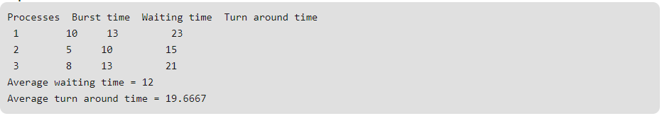
    int processes[] = { 1, 2, 3}; 
    int n = sizeof processes / sizeof processes[0]; 
  // Burst time of all processes 
    int burst_time[] = {10, 5, 8}; 
  
    // Time quantum 
    int quantum = 2; 
    findavgTime(processes, n, burst_time, quantum); 
    return 0; 
} 

• 

Advantages

1. It may be really implementable within the system as a result of it’s not reckoning on the burst time.
2. It doesn’t suffer from the problem of starvation or convoy effect.
3. All the jobs get a fare allocation of central processing unit

Disadvantages

• The higher the time quantum, the higher the response time within the system.
• The lower the time quantum, the higher the context switching overhead within the system.
• Deciding a ideal time quantum is really a very difficult task in the system.

Follow My Blog

Get new content delivered directly to your inbox.